Battery Parameter Extraction in the OpenEPT Data Analyzer
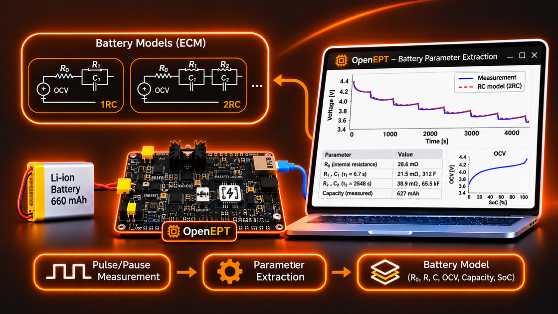
Accurate battery modeling is essential for various functionalities of battery-powered embedded systems. Battery models provide the foundation for estimating its state of charge (SoC), predicting its remaining operational lifetime, and monitoring its condition. Among the commonly used approaches are equivalent circuit models (ECMs), which represent a battery using an open-circuit voltage (OCV) source, an ohmic resistance, and one or more resistor-capacitor (RC) branches that describe its dynamic voltage response.
However, using these models requires determining their parameters for a particular battery. OpenEPT provides a systematic way to extract these parameters from experimental measurements, using a sequence of controlled current pulses separated by rest periods. By analyzing the resulting voltage response, OpenEPT can determine the battery's internal resistance, RC branch parameters, and open-circuit voltage at different states of charge.
This post explains the mathematics behind the battery parameter extraction process and how it is implemented in the OpenEPT software. As with our previous Data Analyzer tutorial, the implementation is divided into a back-end, responsible for processing measurement data and extracting model parameters, and a front-end, which presents the results and provides tools for their analysis. The post first builds the mathematical foundations of the extraction procedure, then shows how the procedure is carried out in OpenEPT on a concrete battery, and finally presents the extracted parameters of that battery. If you have not yet read the overview, start with Inside the OpenEPT Data Analyzer Window.
Throughout this post, the extraction procedure is demonstrated using experimental measurements obtained from a GaoNeng lithium-ion battery with a declared capacity of 660 mAh. The battery was subjected to a pulse/pause discharge procedure, and the recorded measurements were processed using the OpenEPT Data Analyzer. All tables, graphs, and examples presented in this post originate from this single measurement.

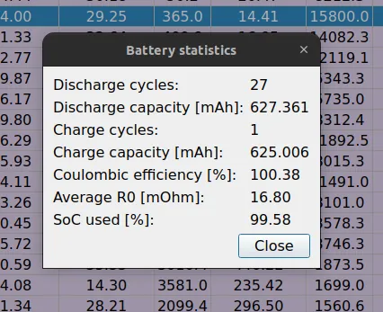
Interestingly, the measurements revealed that the battery delivered approximately 627 mAh, compared to its declared capacity of 660 mAh. This difference illustrates another important benefit of battery characterization: the ability to evaluate actual battery performance rather than relying exclusively on manufacturer specifications. Although a lower measured capacity does not necessarily indicate battery degradation or an inaccurate capacity rating, it may provide an indication of aging, previous usage, or differences between the actual operating conditions and those used to determine the rated capacity.
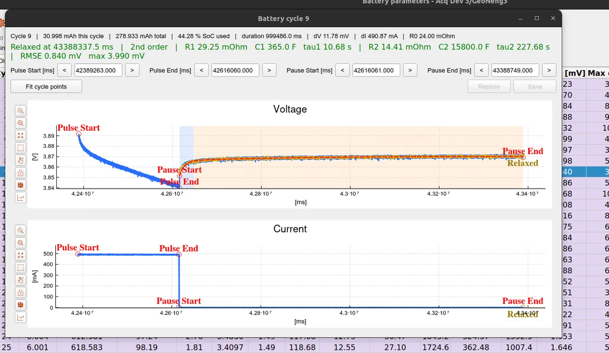
The battery parameter extraction is part of the open-source OpenEPT GUI.
In This Post
- The Model
- The Math, Step by Step
- Fit Quality and the Fit Interval
- Extraction in Practice: Measurement and OpenEPT
- The Extracted Battery Parameters
The Model
OpenEPT fits a Thevenin equivalent circuit to the battery. In its second-order form it consists of:
- an open-circuit voltage
OCV, the rested terminal voltage at the current state of charge; - an ohmic resistance
R0, the instantaneous voltage jump when the current changes; - a fast RC branch
R1 ‖ C1, with a short time constantτ1 = R1·C1; - a slow RC branch
R2 ‖ C2, with a longer time constantτ2 = R2·C2.
During a rest after a discharge pulse, the terminal voltage relaxes back toward OCV as the two RC branches discharge:
where t is time measured from the start of the rest, and A_fast, A_slow are the voltages left on the two branches when the pulse ended. The first-order model is the same expression with only the fast branch. Extraction is the inverse problem: given the measured v(t), recover OCV, R0, R1, C1, R2, C2.
The Math, Step by Step
The whole procedure works on one pulse/pause cycle: a discharge current pulse, delimited by the markers Pulse Start and Pulse End, followed by a pause (a rest at zero current), delimited by Pause Start and Pause End. The pulse produces the ohmic jump that gives R0, and during the pause the voltage relaxes toward the open-circuit voltage, which is what the RC branches and the OCV are read from. The next section shows how such cycles are generated and measured; here we assume one cycle is available and derive its parameters. Everything below is for a single cycle, as implemented in BatteryParamsExtraction::analyzeCycle().
R0, the ohmic resistance
The ohmic resistance is the instantaneous part of the response: the voltage step that appears the moment the pulse ends, before any RC branch has had time to relax. It is read directly from the step between the end of the pulse and the start of the pause:
In the code these are deltaVoltage, deltaCurrent and resistance on the cycle, computed from the samples at the Pulse End and Pause Start markers. R0 is only reported when ΔI is non-zero (resistanceValid).
The averaged pause and the OCV
Real samples are noisy, so before the RC fit the pause is optionally smoothed with a moving average whose width is a setting (Fit average window, in points; a width of 1 keeps the raw samples). The average is anchored at the ends: it is a single sample at Pause Start, grows symmetrically to the full window in the middle, and shrinks back to a single sample at Pause End, so the averaged curve starts exactly on the Pause Start point and introduces no time offset.
The open-circuit voltage is the voltage the cell would settle at if left to rest forever. It is estimated as the average of the last few samples of the fit interval, the settled tail, with the number of points controlled by the OCV window setting:
Averaging the tail instead of taking a single last sample keeps a noisy sample, or the onset of the next pulse right after Pause End, from pulling the value off.
Relaxation detection (dV/dt)
How far the cell has relaxed is decided by a dV/dt criterion: the cell counts as relaxed once the voltage stays within a small band (relaxation threshold, in mV) over a sliding time window (relaxation window, in seconds), after an optional pre-filter. The point where this first happens is the relaxation point.
This search is implemented by BatteryParamsExtraction::relaxationPositionGet() and is the exact same routine the live acquisition uses to decide when to end a pause early, so an offline analysis and a live run agree on where the cell relaxed.
The overpotential and the fit model
With OCV known, define the overpotential, the total voltage left on the RC branches at the start of the pause:
This η is the sum of the two branch amplitudes. Working with the decay rather than the voltage makes the fit a sum of pure exponentials that starts at η and decays to zero:
If η is essentially zero (the cell barely moved during the pulse) there is nothing to fit, and the cycle is reported as such.
Exponential peeling: separating the time constants
Two exponentials with different time constants are separated by peeling, exploiting the fact that late in the pause only the slow branch is still moving:
- Slow branch. Fit a single exponential to the later part of the decay (from a split point to the end). Because the fast branch has already vanished there, this returns the slow time constant
τ2and its amplitude. - Residual. Subtract that slow exponential from the early part of the decay.
- Fast branch. Fit a single exponential to the residual, returning the fast time constant
τ1.
Each single-exponential fit is a logarithmically spaced grid search over the time constant with a few refinement passes, implemented by an internal helper. For a fixed τ the best amplitude is linear and solved in closed form, and the fit error is obtained algebraically from the same sums, so no second pass over the samples is needed. For a long pause the number of fit points is capped, which keeps the search fast without changing the recovered time constants.
If the slow fit fails or the two time constants are not well separated, the model gracefully falls back to a single (first-order) branch.
Anchored amplitudes
The time constants come from the peel, but the amplitudes are re-solved jointly under a physical constraint: the two branches must add up to the overpotential, so the fitted curve starts exactly at the Pause Start voltage and settles exactly on the OCV:
With τ1 and τ2 fixed, this is a one-parameter least-squares problem; the code solves for A_fast in closed form and sets A_slow = η - A_fast, clamping the result so neither amplitude flips sign. Anchoring the amplitudes this way keeps the two branches physically meaningful instead of letting the fit trade one off against the other.
From amplitudes to R and C
The amplitudes above are the voltages seen on the branches at the start of the pause. They are not yet I·R, because during a pulse of finite duration a branch only charges part way toward its steady value. A branch with time constant τ driven for a pulse of duration Tpulse reaches a fraction
of its steady I·R. Inverting this gives the branch resistance and capacitance from its amplitude and time constant:
applied with I the pulse current and the matching charged factor for each branch. The code computes R1, C1 from the fast branch and R2, C2 from the slow branch exactly this way.
When a branch does not exist
Not every relaxation contains two distinct time constants. When the joint re-solve assigns (almost) no amplitude to a branch, that branch cannot be determined, and OpenEPT leaves its R and C empty rather than reporting a misleading zero. The fast branch stays in the R1/C1 slot, the slow branch in R2/C2, and a per-branch validity flag (r1Valid, r2Valid) records which ones were actually identified. A relaxation that is a single slow exponential therefore shows R2/C2 and an empty R1/C1, with a short note explaining why.
State of charge
To place each cycle on a state-of-charge axis, the charge drawn out of the battery is integrated from the measured current, cycle by cycle:
capacity is the battery's declared capacity and SoC_initial the starting state of charge (both are settings). With a state of charge attached to every cycle, the extracted R0, R1, R2, C1, C2 and OCV can be plotted against SoC across the whole discharge, which is exactly the result shown at the end of this post.
Fit Quality and the Fit Interval
After the model is built, its quality is reported over the whole pause, independent of where the parameters came from:
Two fit intervals are offered. Pause start to relaxation point fits only up to the point where the cell relaxed, leaving out a tail that is still slowly moving; Pause start to pause end uses the whole pause. When the relaxation point is not reached within the pause, both intervals fall back to the pause end so a model and an OCV are still produced. The fit interval, the model order, the window widths and the capacity all live in a settings structure (batteryparams_settings_t) that can be saved with the profile.
Extraction in Practice: Measurement and OpenEPT
With the mathematics in place, this section shows how the procedure is actually carried out: how the pulse/pause data is produced, where the math lives in the code, and the tools the Battery parameters window offers for working with the results. Everything here is from the GaoNeng recording.
The pulse/pause measurement
To make the extraction well-posed, the battery is discharged with a repeating cycle: a current pulse of known amplitude and duration, followed by a pause during which no current flows and the voltage relaxes. Four markers delimit each cycle:
- Pulse Start / Pulse End, the discharge pulse,
- Pause Start / Pause End, the rest period.
These markers are produced by the "Bat Param Extraction" load mode and stored with the recording, exactly like any other energy point marker. The extraction processes one cycle at a time: the pulse gives R0, and the pause gives the RC branches and the OCV. As the discharge progresses, every cycle sits at a slightly lower state of charge, so the sequence of cycles traces how the parameters change across the whole discharge.
Back-End: where the math lives
All of the mathematics above is implemented in one processing class, independent of the GUI:
The single most important function is BatteryParamsExtraction::analyzeCycle(), given one cycle's samples and markers plus a settings structure, it fills in R0, R1, C1, R2, C2, OCV, the time constants, the fit error and the validity flags. Every equation from the previous sections happens inside it.
The windows that present the results are:
- batteryparamswnd.cpp, the main battery parameters window (the per-cycle table, the graphs, the analyses),
- batterycyclewnd.cpp, the single-cycle inspector.
The analysis of each cycle is run on a worker thread so the interface never blocks, and when many cycles are analyzed at once the work is spread across all CPU cores.
The Battery Parameters Window
The results of the extraction are presented in the Battery parameters window (BatteryParamsWnd). It is organized around a tool bar, a per-cycle table, and a set of windows reached from the tool bar.
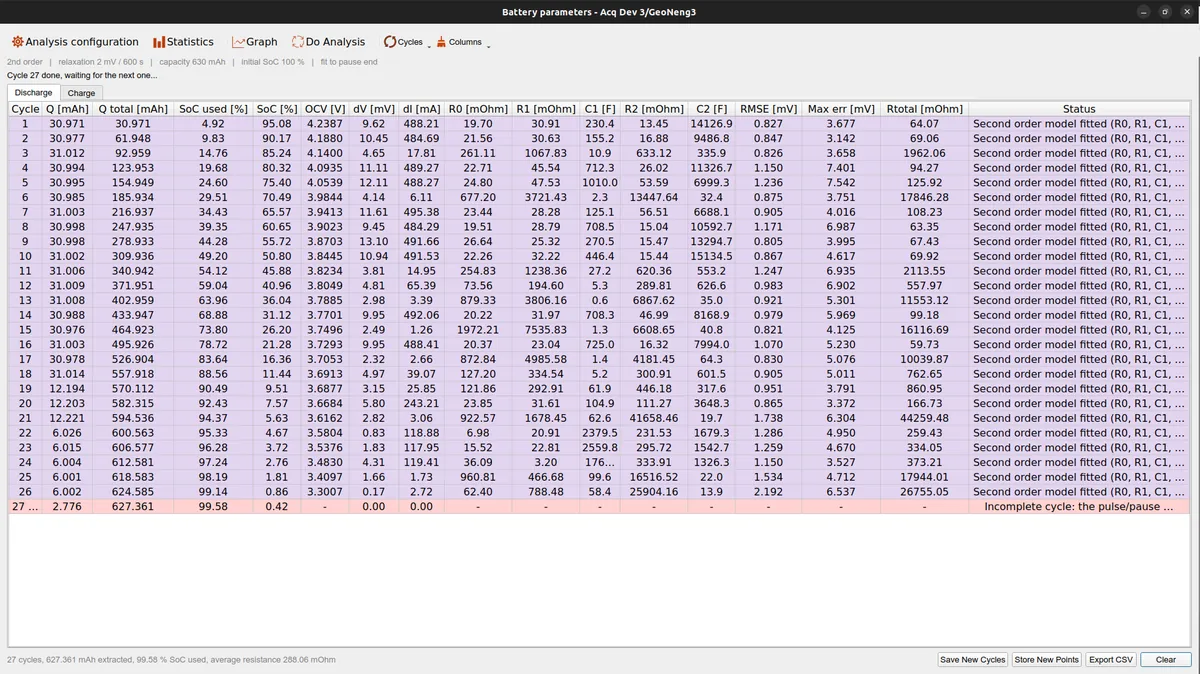
The tool bar collects everything that acts on the whole set of cycles:
- Analysis configuration opens the settings dialog (model order, relaxation criterion, fit interval, the fit-average and OCV window widths, the capacity and the initial state of charge). The line right below the tool bar always echoes the active settings.
- Statistics opens a summary of the whole discharge.
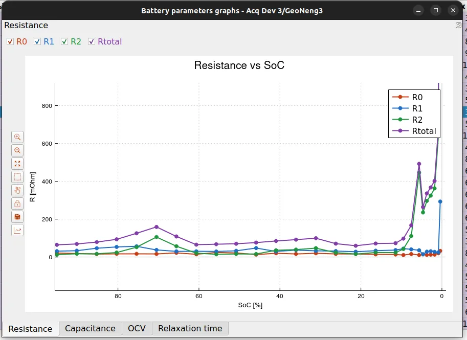
- Graph opens the parameter-versus-SoC graphs.
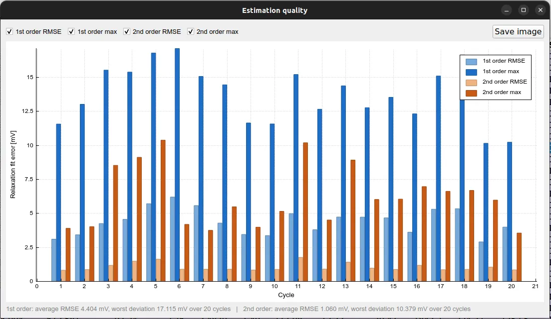
- Do Analysis groups the deeper analyses (OCV analysis, estimation quality, fit interval comparison).
- Cycles holds the operations that recompute or adjust the cycles.
- Columns lets you choose which columns of the table are shown.
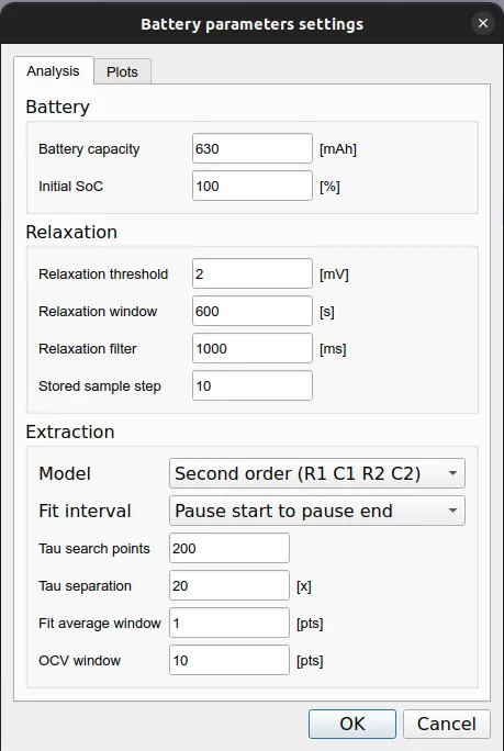
The settings behind the whole extraction live in the Analysis configuration dialog: the battery capacity and initial state of charge, the relaxation criterion and sample decimation, and the extraction options (model order, fit interval, the tau search grid, and the fit-average and OCV window widths). These are the same settings used throughout the math above, and they can be saved with the profile.
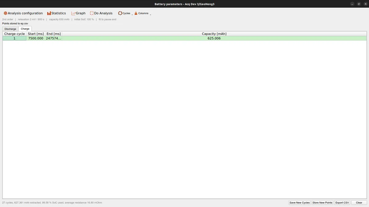
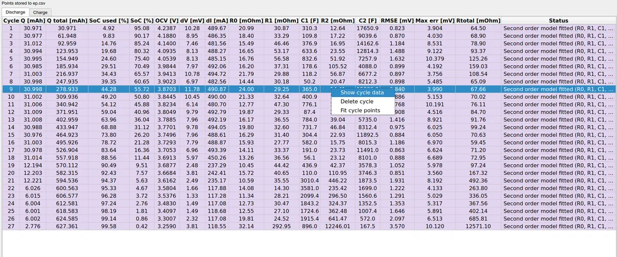
The per-cycle table has a Discharge and a Charge tab. Each discharge row is one cycle with its R0, R1, C1, R2, C2, OCV, state of charge, errors, and a status that spells out what was fitted. Rows are colored by outcome, and a cycle whose pulse/pause markers were not all captured is marked as incomplete and left out of the fit. The Charge tab accounts for the charge phases instead: each charge cycle with its start, end and the capacity put back into the battery, which is what the coulombic efficiency is computed from.
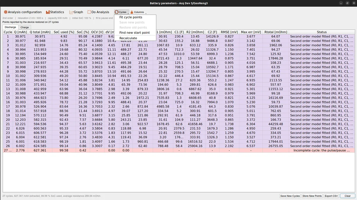
The Cycles menu carries the per-cycle operations: Fit cycle points snaps the Pulse End and Pause Start markers onto the settled levels around the current step, Find new start point sweeps the pause start to minimize the fit error, Recalculate re-runs the analysis with the current settings, and Save / Restore points keep or revert the adjustments.
Right-clicking a cycle opens a context menu to show that cycle's data in the single-cycle inspector, delete it, or fit its points.
The Statistics window summarizes the whole discharge: the number of discharge and charge cycles, the discharge and charge capacities, the coulombic efficiency, the average R0, and the state of charge used. For the GaoNeng cell this is where the measured capacity of about 627 mAh is read off.
Do Analysis opens the deeper comparisons. The estimation quality view, for example, fits both the first and the second order model to every cycle and plots their RMSE and worst-case error side by side, which shows at a glance whether the second RC branch is worth keeping for a given battery.
Each heavy operation in this window (recalculating, fitting the points of every cycle, sweeping the start point) runs on a worker thread and, when there are many cycles, is spread across all CPU cores, so the window stays responsive while the analysis runs.
The Extracted Battery Parameters
Running the whole procedure on the GaoNeng cell turns its pulsed discharge into a complete, state-of-charge-dependent model. Plotting each extracted parameter against the state of charge shows how the battery behaves as it empties: the resistances stay low and flat through most of the discharge and climb steeply near the end, while the open-circuit voltage traces the familiar discharge curve.
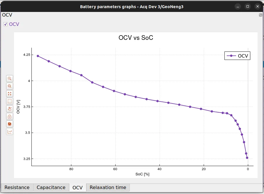
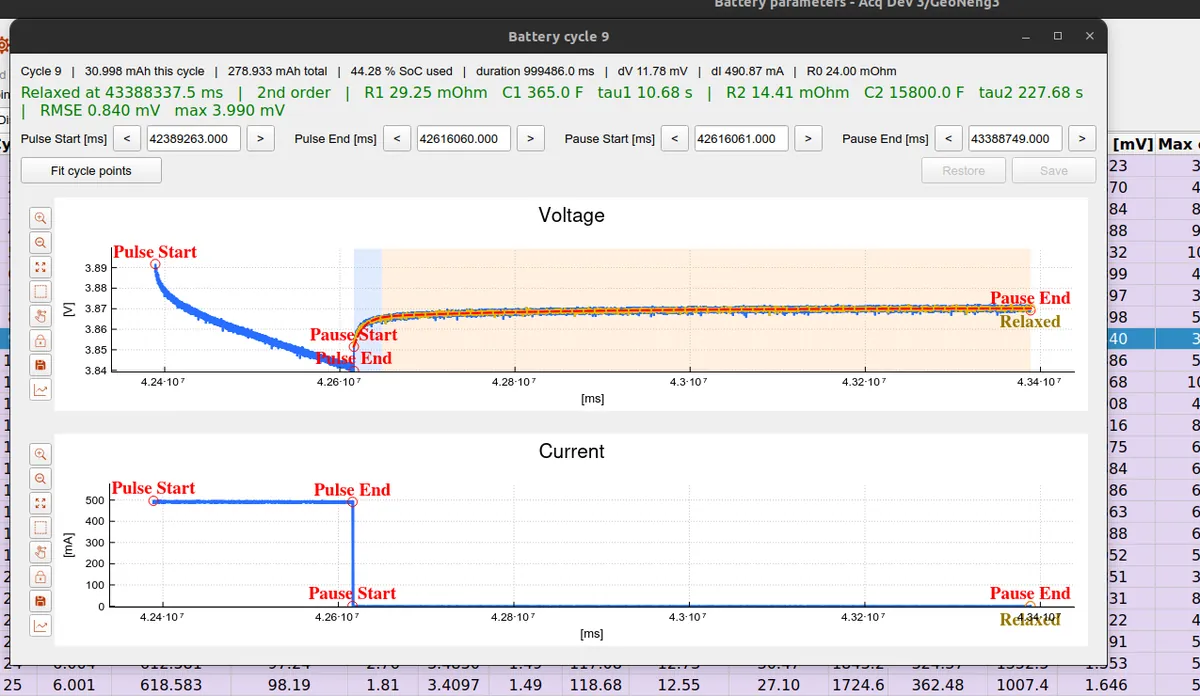
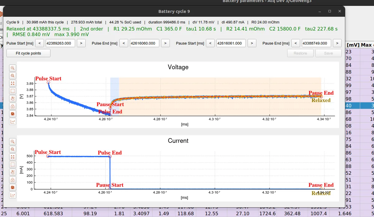
Not every cycle yields both RC branches. On the GaoNeng cell, cycles whose relaxation is dominated by a single time constant are reported as first order, with the missing branch left blank rather than shown as zero. Opening such a cycle in the single-cycle inspector shows exactly what that means.
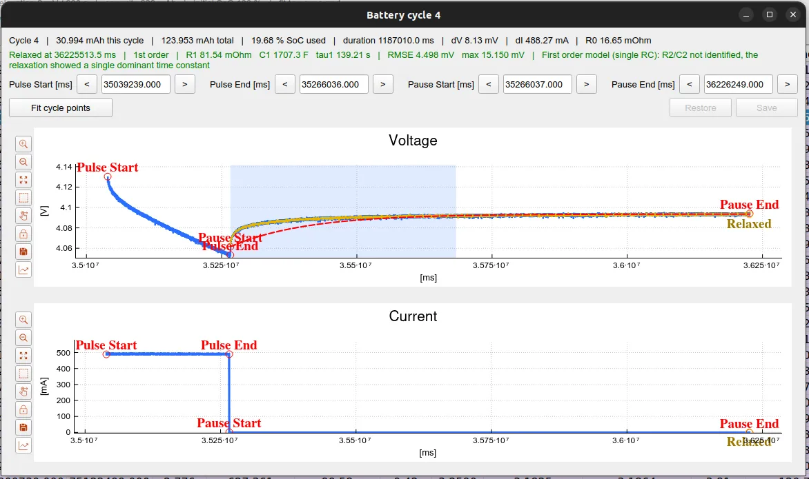
This is cycle 4 of the GaoNeng discharge. The top line summarizes the cycle itself: it moved 30.994 mAh of charge (123.953 mAh cumulatively), which corresponds to 19.68 % of the cell's usable capacity, over a pulse of about 1187.0 s. The two plots below are the raw measurement the extraction works on. The current plot shows the shape the whole method relies on: a flat discharge pulse of dI = 488.27 mA between Pulse Start and Pulse End, then zero current through the pause that follows. The voltage plot shows the battery's response to that step, with the fitted model (red dashed) drawn over the measured samples (blue).
Reading the parameters off this one cycle follows the same three moves described earlier in the post:
R0from the ohmic jump. The instant the current drops to zero at Pulse End, the terminal voltage jumps up bydV = 8.13 mVbefore any RC branch has had time to move. That step divided by the current gives the ohmic resistance directly,R0 = dV / dI = 8.13 mV / 488.27 mA = 16.65 mΩ— exactly the value shown in the header.- The relaxation, fitted over the shaded window. After the jump, the voltage keeps climbing more slowly toward the open-circuit voltage as the RC branches discharge. OpenEPT fits this curve over the highlighted relaxation band and marks the point where it is considered settled (Relaxed, here at
36225513.5 ms). The fit tracks the measurement closely:RMSE 4.498 mV, with a worst-case error of15.150 mVat the very start of the relaxation, where the response changes fastest. - A single RC branch is enough. The relaxation here is one clean exponential rather than a fast-then-slow pair, so the fit resolves only one branch:
R1 = 81.54 mΩandC1 = 1707.3 F, giving a time constantτ1 = R1 · C1 = 139.21 s. The slow branch finds no amplitude to explain, so OpenEPT reports "R2/C2 not identified, the relaxation showed a single dominant time constant" and leavesR2 / C2blank — the first-order outcome of the branch-validity logic described above, not a fitted zero.
The Pulse Start / End and Pause Start / End fields let the boundaries be nudged by hand and the cycle re-fitted with Fit cycle points if a marker landed poorly, and Save writes the corrected values back; on this cycle the automatic markers already sit where they should, so no adjustment is needed.
Taken together, the per-cycle table, the single-cycle inspector and the parameter-versus-SoC graphs turn the pulsed discharge of the GaoNeng cell into a complete, state-of-charge-dependent equivalent-circuit model of the battery, all from data the OpenEPT Energy Profiler Probe records on its own.