Consumption Analysis in the OpenEPT Data Analyzer
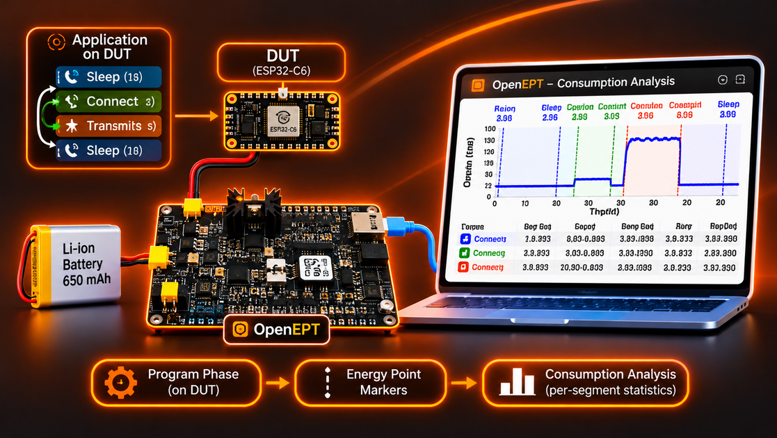
A recorded consumption profile is a long dataset of voltage and current measurements. On its own it answers the question "how much did the device draw?" only after a lot of manual zooming and reading. The consumption analysis in the OpenEPT Data Analyzer turns that waveform into numbers you can act on: how much energy and charge each phase of the program consumed, how long each phase lasted, and how the current and voltage behaved inside it.
This post follows the consumption analysis from both sides. The back-end section explains how a profile is parsed and how the statistics are computed, and points to the exact place in the source where each step is implemented. The front-end section walks through every element of the interface and what it can do. If you are new to the Data Analyzer itself, start with Inside the OpenEPT Data Analyzer Window.
The consumption analysis is part of the open-source OpenEPT GUI.
In This Post
The Idea: Segments Between Markers
Consumption analysis starts from energy point markers: named instants on the time axis, stored in the profile's ep.csv file. They are usually sent by the device under test during an acquisition, but they can also be added afterwards, synthetically, from the Load tab. Two markers that share a name, <name> Start and <name> Stop, enclose a segment. A segment is the part of the recording that belongs to one phase of the program under test, such as Sleep Start / Sleep Stop or Transmit Start / Transmit Stop. A marker without a partner stays a point marker: it labels a moment but has no duration.
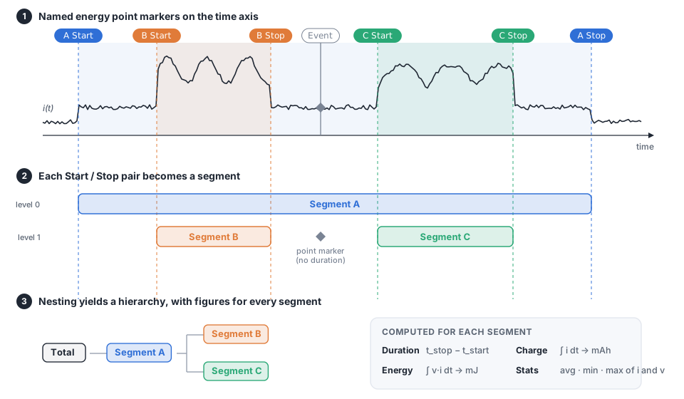
For each segment, the analysis integrates the current and power over its time span and records the extremes of current and voltage inside it. Segments may also be nested: one pair can open and close entirely inside another, before the outer Stop arrives. So the result is a hierarchy of segments rather than a flat list, and it follows the structure of the program that produced the data.
Where the Markers Come From
The segments only exist because the device under test marks the boundaries of its own program phases. In OpenEPT these boundaries are energy point markers, and a dedicated mechanism carries them from the device to the GUI with sample-accurate timing. All the examples in this post were produced by an ESP32-C6 running on the OpenEPT Compact Low Power board, and its markers are what split the recording into the WiFi, server, upload, compute and sense phases seen later.
Sending markers with FEPLib
On the device side, markers are emitted with FEPLib, the OpenEPT embedded-device library that a device under test links against.
FEPLib exposes a small API: OpenEPT_ED_Init(), OpenEPT_ED_Start() / OpenEPT_ED_Stop() to open and close the link, and OpenEPT_ED_SetEPFast(name, size) to place a marker. On the wire every message is a single-character header, a colon, the payload, and a carriage return:
0:START\r/0:STOP\r, open and close the link (each acknowledged by the acquisition device withOK\r),1:<name>\r, an energy point marker,2:<message>\r, a plain info message.
The important detail is how a marker is placed in time. It does not rely on when the name bytes happen to arrive, which is subject to UART and buffering latency. Instead, SetEPFast first toggles a dedicated SYNC line and only then sends the name:
int OpenEPT_ED_SetEPFast(uint8_t* epName, uint32_t epNameSize)
{
    OpenEPT_ED_Platform_SyncToogle();          // hardware edge = the marker's timestamp
    OpenEPT_ED_Platform_Send('1');             // "1:" energy-point header
    OpenEPT_ED_Platform_Send(':');
    for (uint32_t i = 0; i < epNameSize; i++)
        OpenEPT_ED_Platform_Send(epName[i]);   // the marker name
    OpenEPT_ED_Platform_Send('\r');
    return OPEN_EPT_STATUS_OK;
}
The SYNC edge is a hardware event the acquisition device can timestamp to the exact sample, while the name arrives over the serial link a moment later; associating the two gives a marker that is placed precisely even though its name was transmitted asynchronously. On the ESP32-C6, FEPLib's platform layer wires this to real peripherals: the name goes out on UART1 (TX 20, RX 21) at 115200 baud, and the SYNC line is GPIO 19, toggled with a single gpio_set_level().
FEPLib is intentionally a very small library, and the device under test is not required to use it. The probe never sees which library the DUT runs. It only sees the signals on the wire, so any firmware works as long as it follows the same format:
- toggle the SYNC line at the instant the marker should land, then send the name,
- frame every message as
<header>:<payload>\r, with0for control,1for an energy point and2for info, - open and close the session with
0:START\r/0:STOP\rand wait for theOK\racknowledgment.
Think of FEPLib as a reference implementation of this format rather than a dependency. You can link it directly, port its few functions to another platform, or write the same messages from your own code in any language or RTOS.
Support in the OpenEPT firmware
The matching half of this mechanism lives in the OpenEPT acquisition firmware, the Energy Profiler Probe (EPP), the STM32-based device that samples the voltage and current. Marking points on an acquisition is not new to the EPP: an earlier version already had a simple energy-point input. It was a single hardware push-button on the probe. Pressing it captured the index of the sample being acquired at that instant and emitted one breakpoint. That was enough to drop a manual flag on the waveform by hand, but nothing more. The device under test could not name its own points, bracket a phase, or drive the link; every marker was an anonymous, operator-initiated instant.
For the consumption analysis described here, that input was rebuilt into a full energy-point link, an Energy Debugger service that understands the FEPLib protocol end to end. The physical button still works and still feeds the same pipeline, but it is now only one source among several. The service adds the following new functionality:
- A typed FEPLib protocol parser on the serial input. A UART receive interrupt (on the EPP's dedicated UART4 energy-point port) assembles each incoming message and classifies it by its single-character header:
0:→ a CONTROL message,1:→ an energy point (EP),2:→ an INFO message. The two-character header is stripped and the payload is queued for the service task. - Named energy points. An EP message carries a text name (
WiFi Con Start,TX,Compute Stop, …), so markers are no longer anonymous button presses but named instants the GUI can label, pair into segments, and nest. - SYNC-edge capture decoupled from the name. A change on the SYNC pin triggers an interrupt that captures the exact sample position (
packetId+sampleId) straight from the acquisition stream, independent of when the name bytes arrive. The service then pairs that captured position with the next queued name to assemble one complete energy point, so a marker lands on the correct sample no matter how busy or delayed the serial link is. - A START/STOP handshake.
0:STARTand0:STOPCONTROL messages arm and disarm the link and are each acknowledged withOK\r;STARTalso resets the position queue. This lets the DUT bracket a whole measurement session and keeps names and sample positions in step across the DUT's own sleep/wake cycles. - An INFO channel.
2:messages are forwarded to the GUI's status link, so the device can annotate a recording with plain text (firmware version, a tag, a warning) alongside the markers. - Firmware-generated markers. A new API,
ENERGY_DEBUGGER_MarkFromISR(name, length), lets the acquisition firmware itself emit a named breakpoint from an interrupt, equivalent to a button press followed by a name, so points can be raised from firmware events, not only from the button or the DUT. - Energy points carried onto the waves. Because each point travels with its
packetIdandsampleId, the GUI can place it on the exact sample of the voltage and current waveforms. Points that arrive while no acquisition is running are counted as dropped rather than mis-placed, and a completed point is fanned out over TCP to every connected GUI.
The acquisition-side link is the Energy Debugger service:
- energy_debugger.c:
prvEDEBUGGING_SerialCharReceived()(UART4 header parser,0:/1:/2:→ CONTROL/EP/INFO),prvEDEBUGGING_ButtonPressedCallback()(SYNC/button capture ofpacketId+sampleId), the service task (START/STOP handshake, name↔position pairing, TCP fan-out) - energy_debugger.h:
ENERGY_DEBUGGER_Init(),ENERGY_DEBUGGER_CreateLink(),ENERGY_DEBUGGER_MarkFromISR()
Forming Start/Stop markers on the DUT
A single SetEPFast call places one named instant; a segment needs two, a <name> Start and a <name> Stop. The device under test forms them by sending the two names around the code it wants to measure. In the ESP32-C6 example this is wrapped in small helpers:
static void ep(const char *name)
{
    OpenEPT_ED_SetEPFast((uint8_t*)name, strlen(name));
}

static void epStart(const char *segment)       // sends "<segment> Start"
{
    char buffer[64];
    snprintf(buffer, sizeof(buffer), "%s Start", segment);
    ep(buffer);
}

static void epStop(const char *segment)        // sends "<segment> Stop"
{
    char buffer[64];
    snprintf(buffer, sizeof(buffer), "%s Stop", segment);
    ep(buffer);
}
Wrapping any operation between epStart and epStop turns it into a measurable segment:
epStart("WiFi Con 1");     // "WiFi Con 1 Start"
wifi_connect();
epStop("WiFi Con 1");      // "WiFi Con 1 Stop"
The example program, an ESP32-C6 running a realistic IoT workload, brackets every phase this way: connecting to WiFi and a server, sending Hello and TX packets during Upload, running fft, filter, matrix and crc inside Compute, acquiring in Sense, and dropping into Light LP / Deep LP low-power states. Nesting is natural, an inner TX pair sits inside an outer Upload pair, and that nesting is exactly what the statistics window later shows as a tree.
The ESP32-C6 firmware dataflow
To see where all these markers actually come from, it helps to look at the use-case firmware as a whole. The ESP32-C6 on the Compact Low Power board runs a duty-cycled IoT workload: it wakes, does a burst of real work (connect, sense, compute, exchange data with a server), then drops back into a low-power state and sleeps until the next cycle. That shape, a short active window surrounded by sleep, is exactly what a consumption profile is meant to capture, which is why it is used as the example throughout this post.
The dataflow is deliberately one-directional and lightweight. At start-up the firmware calls OpenEPT_ED_Init() and then OpenEPT_ED_Start(), which runs the 0:START handshake with the acquisition probe. From then on, the only energy-profiling data the ESP32 produces is a stream of SYNC edges and named markers: every program phase is wrapped between an epStart / epStop pair (an epIdStart / epIdStop variant appends a cycle number so repeated phases stay distinct), and each call toggles the SYNC line and sends its 1:<name> over the UART. The firmware never has to measure or report current itself. The probe turns the voltage and current it samples on the battery into the actual consumption data, and the markers simply tell it where each phase begins and ends. When the firmware enters deep sleep it sends 0:STOP and powers down; after the timer wakes it, it re-runs 0:START so names and sample positions line up again across the sleep boundary.
A single active cycle walks through a small state machine: boot and bring-up, WiFi connect, server connect, the services pipeline (Sense → Compute → Upload → KeepAlive → Download → Report), then teardown and a low-power state. Even cycles take a short Light LP sleep and loop straight back into the next active window; odd cycles take a full Deep LP sleep that powers the chip down and restarts it on the timer. If a cycle gets stuck, a time-out resets the device through deep sleep. The markers emitted at each step are what later appear in the GUI as the segment tree:
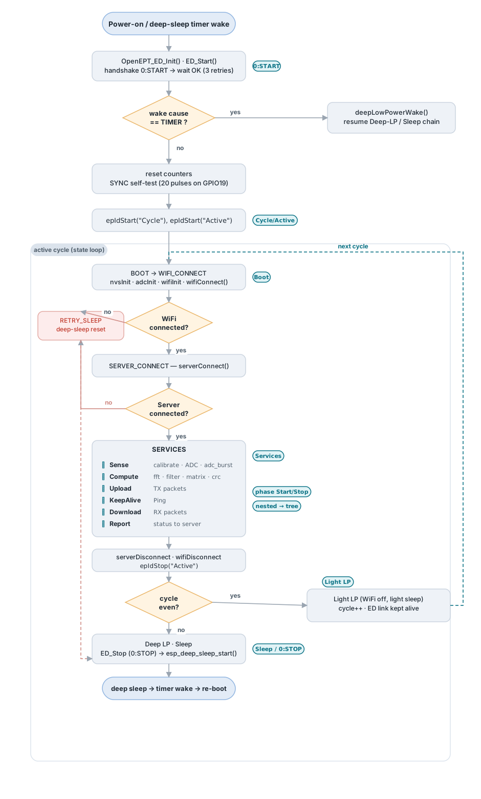
The use-case firmware is the ESP32-C6 application in the Testing project. The state machine and the ep / epStart / epStop helpers are in its main.c; the SYNC and UART wiring is in the FEPLib platform layer (platform_esp32.c).
Receiving and showing the markers in the GUI
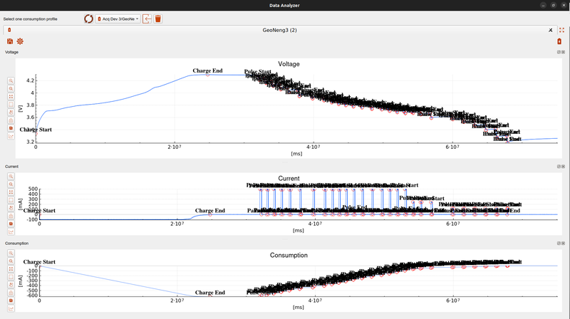
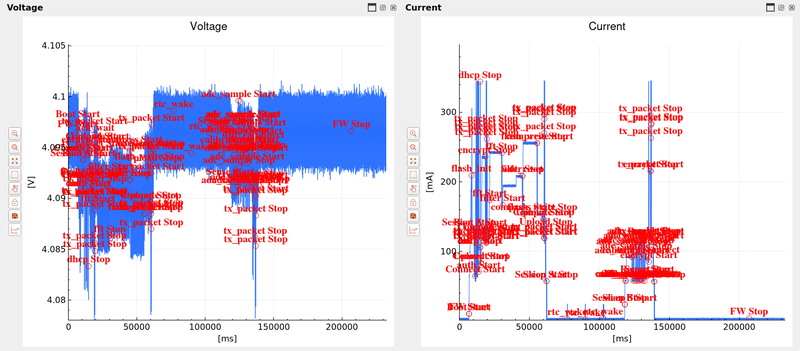
On the OpenEPT side, each energy point that arrives during an acquisition is timestamped against the sample stream, stored in the profile's ep.csv file next to the voltage and current samples, and, when the profile is opened in the Data Analyzer, drawn directly on the three plots. A Start and its matching Stop bracket the phase they name, so the program's structure is visible on the raw waveform before any statistics are computed.
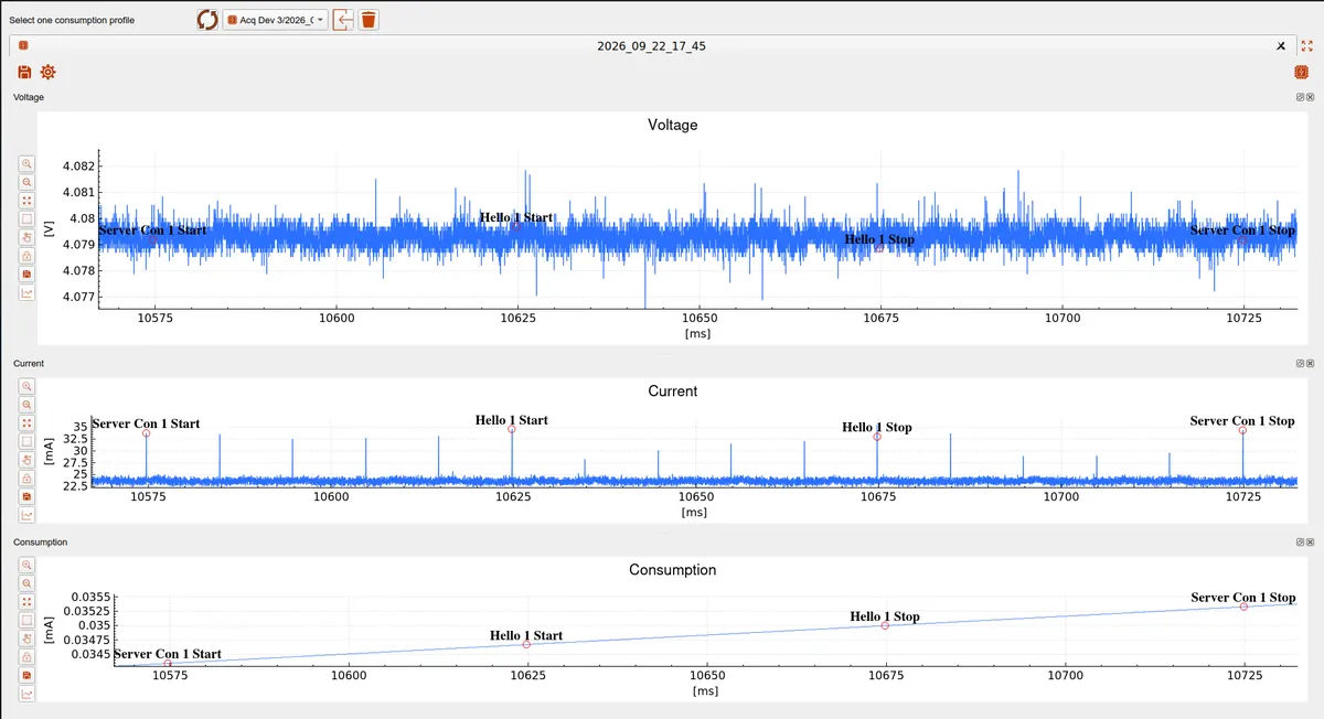
From here the markers are exactly the input the consumption analysis works on: the back-end pairs each Start with its Stop to build the segments, as described next.
Back-End
Loading the profile
Before anything can be analyzed, the three data files of the profile have to be read into memory. This is done by the DataAnalyzerWorker, which runs on its own thread so the interface never blocks. The three files are independent, so they are parsed concurrently:
vc.csv, voltage and current samples, byparseVCData(),cons.csv, accumulated consumption, byparseConsumptionData(),ep.csv, the energy point markers, byparseEPFile().
Loading and parsing are implemented in:
- dataanalyzer.cpp,
DataAnalyzerWorker::processVoltCurConData(),parseVCData(),parseConsumptionData(),parseEPFile() - dataanalyzerworker.h
The parsed samples and markers are received by the profile window in dataanalyzerprofile.cpp (processingVolCurConDone(), processingEPDone()).
Once parsing finishes, the profile window keeps the full voltage and current vectors (and their time axes) in memory. These are the arrays the statistics are later computed over.
From markers to segments
The markers in ep.csv are just named points in time. Turning them into segments is a matching problem: every <name> Start has to be paired with the next matching <name> Stop. Two helper functions recognize the two halves of a pair:
DataAnalyzerStatisticsWorker::markerIsStart(), returns true, and the bare segment name, for a"<name> Start"marker;DataAnalyzerStatisticsWorker::markerIsStop(), the same for a"<name> Stop"marker.
Walking the ordered list of markers and matching starts to stops yields, for each segment, a start index and an end index into the sample arrays, plus a parent index when one segment opens inside another. Markers that never pair up are reported back to the user as warnings rather than silently dropped. Single markers that are neither a start nor a stop are kept as point markers, named instants without a duration.
Each segment is stored in a dataanalyzer_segment_stat_t, which holds its name, its start/end indices and times, its parent, and the figures computed for it.
Computing a segment
The numbers for one segment are computed by DataAnalyzerStatisticsWorker::computeSegment(). It is a single pass over the samples between the segment's start and end indices that accumulates four integrals and tracks four extremes:
for(int i = startIndex; i < endIndex; i++)
{
    double dt = keys[i + 1] - keys[i];       // sample interval
    chargeMAms += current[i] * dt;           // charge    (mA x ms)
    energyUJ   += voltage[i] * current[i] * dt; // energy (uJ)
    currentSum += current[i];
    voltageSum += voltage[i];
    // min / max of current and voltage are tracked here as well
}
From these accumulators the segment's figures are derived:
| Figure | How it is obtained |
|---|---|
| Duration | endTime - startTime |
| Consumption (charge) | chargeMAms / 3 600 000 → in mAh |
| Energy | energyUJ / 1000 → in mJ |
| Average current / voltage | sum divided by the number of samples |
| Min / max current, min / max voltage | tracked during the pass |
Charge is the time-integral of the current, and energy is the time-integral of the instantaneous power v·i; both are computed with the real, possibly non-uniform, sample spacing dt, so irregular sampling does not bias the result. A final total segment aggregates the whole recording the same way.
The statistics computation lives in:
- dataanalyzerstatistics.cpp,
DataAnalyzerStatisticsWorker::onComputeStatistics(),computeSegment(),markerIsStart(),markerIsStop() - dataanalyzerstatistics.h
Threading and progress
The computation also runs off the GUI thread. The profile window emits a request with the voltage, current and marker arrays; the statistics worker, living on its own QThread, computes the segments and reports progress, then returns the per-segment results, the point markers, the total, and any warnings in a single signal. The window only has to display them.
Front-End
The profile window
A profile is opened from the drop-down at the top of the Data Analyzer, where each recording is tagged with an icon that matches its analysis type: the OpenEPT logo for a consumption profile, a battery for a battery profile. Picking a consumption recording opens it as its own tab.
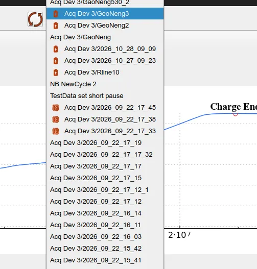
Everything the user then does with that profile starts in the profile window (DataAnalyzerProfile). Across its top sits a small tool bar. For a consumption profile it shows, from left to right:
- Save all plots, export the current view of the three plots as images,
- Profile type (gear), edit the analysis type and metadata of the profile,
- and, pushed to the right, the analysis icon that matches the profile type: for a consumption profile this is Generate statistics (the OpenEPT logo).
Below the tool bar are the three plots.
The plots
The profile shows three stacked, dockable plots, Voltage, Current and Consumption, built with the shared OpenEPT Plot widget. Each plot carries the same vertical tool column used everywhere in OpenEPT:
- Zoom in / Zoom out around the current center,
- Fit to data (expand) to frame the whole recording,
- Zoom area to rubber-band a region,
- Move graph to pan,
- Lock axis to tie this plot's X axis to the other locked plots, so all three stay aligned in time while you zoom and pan,
- Save image to export the plot as PNG or SVG.
Because the three plots share the same time base, locking their axes is what lets you read current, voltage and accumulated consumption at exactly the same instant, as in the marker figure shown earlier.
Energy point markers
The energy point markers from ep.csv are drawn directly on the curves, visible on all three plots in the marker figure shown earlier. Start/Stop pairs annotate the segment they delimit, and standalone points appear as labeled markers. This makes the boundaries of each program phase visible on the raw data before any statistics are computed, and it is the same visual language used for markers that come from a live device.
The statistics window
Pressing Generate statistics runs the back-end described above and opens the statistics window (DataAnalyzerStatisticsWnd). It presents the result as a tree: nested segments appear as child rows of the segment that contains them, mirroring the program structure. Each row (DataAnalyzerStatisticsItem) shows the segment's figures, its first and last action time, consumption, energy and duration, and its share of the cycle and of its parent segment. The final total row summarizes the whole recording.
Alongside the tree, a share bar (DataAnalyzerShareBar) visualizes how the total energy is distributed across the segments: each segment gets a colored slice proportional to its share, using the same color it has on the plots. This answers, at a glance, which phase dominates the energy budget.
The window also lets you show or hide the markers of individual segments on the plots, so a busy recording can be reduced to just the phases you are interested in. If any Start/Stop markers did not pair up, the collected warnings are shown so the mismatch can be fixed in the recording. Each row can be expanded and collapsed, and the Export CSV button writes the whole table out for further processing.
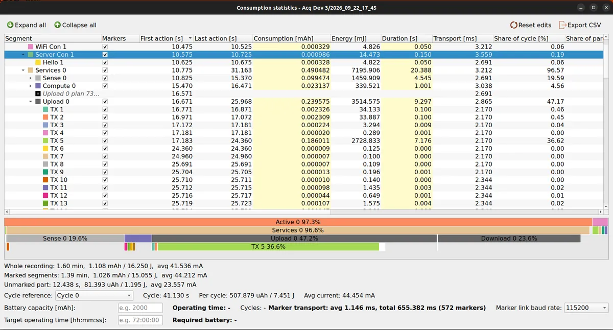
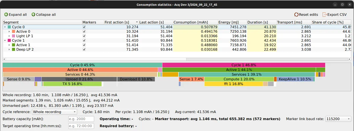
When the program runs in repeating cycles, collapsing the tree to the top level shows one row per cycle, so two cycles can be compared side by side and the share bar splits the recording between them.
Projecting battery life
The bottom of the statistics window turns the measurement into a battery-life estimate. First a cycle reference is chosen: the whole recording, only the marked segments, or one specific cycle. From it the window derives the charge and energy consumed per cycle and the average current.

With a cycle defined, two complementary estimates become available. Entering a battery capacity gives the operating time and the number of cycles that capacity sustains; entering a target operating time gives the required battery capacity instead. Because the per-cycle figures come from a real measurement rather than a datasheet, the projection reflects how the device actually behaves.