Generating Loads with the Energy Profiler Probe
The Energy Profiler Probe (EPP) does not only measure current; it can also draw it. The Load tab of the OpenEPT GUI lets you sink a constant current from a battery or a supply, replay a standard waveform, or build your own current profile chunk by chunk — with random variation and energy point markers that appear on the plots exactly like markers from a real device. This guide walks through the Load tab control by control, the three load modes with measured examples, the waveform library and wave files, and finally what marker-annotated profiles make possible. If you are interested in how it works inside, see Programmable Load: Firmware, Protocol and GUI Implementation.
Everything described here is available in the current OpenEPT GUI release together with the matching EPP firmware, except the Data Analyzer statistics shown in the last section, which are a preview of ongoing work.
Download the Latest GUI Release
Download the Latest EPP Firmware
Ready-made wave files used in this guide: Documentation/Waves
Watch It First
If you would rather see the feature than read about it, two short videos demonstrate everything this guide covers: the first walks through the Load tab, static loads and standard and custom waves; the second adds energy point markers to a wave and shows how they appear on the plots.

Programmable load generator
Static load, standard waves and building a custom current profile in the Load tab.
Programmable load generator with markers
Adding energy point markers to a custom wave and reading them back on the plots.
In This Guide
- Before You Start – wiring, and the four parts of the Load tab that every mode shares.
- Static Load – one constant current, with the measured result.
- Standard Waves – ramp, sawtooth, triangle, square and sine from four numbers; a sine as measured.
- Custom Waves – the chunk table explained column by column; a real device profile replayed.
- Waveform Library and Wave Files – saving, reusing and sharing waves.
- Using a Wave as a Discharge Profile – realistic battery discharge.
- Markers and the Data Analyzer – turning a profile into per-segment numbers.
Before You Start
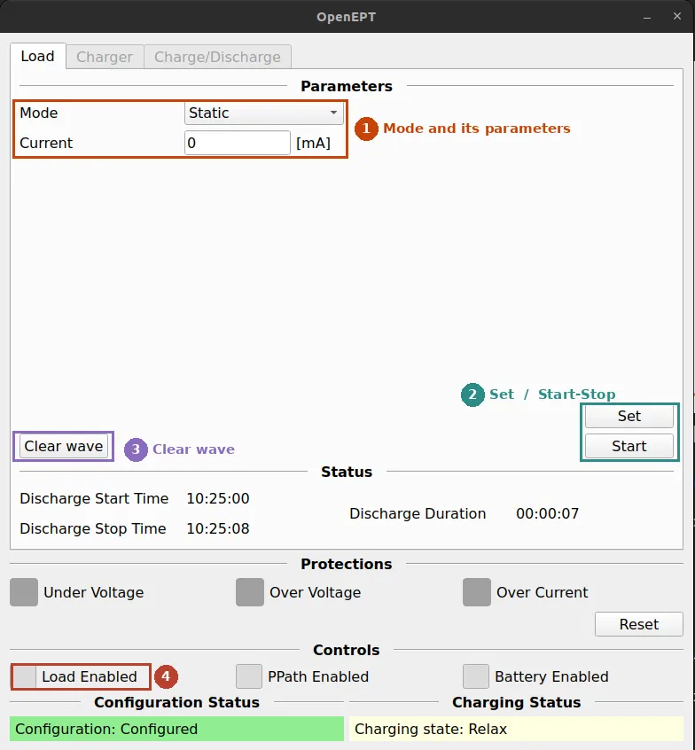
Whatever mode you pick, the tab is always organised the same way:
- Mode and its parameters – the Mode selector switches between Static, Standard Wave and Custom Wave; only the fields below it change. In Static mode there is a single Current entry in mA.
- Set / Start – Set sends the value(s) from frame 1 to the device and stores them there; it does not start anything. Start is what actually makes the device draw current: in Static mode it switches the DAC that drives the sink on, in the wave modes it starts playing the wave. While running, the same button reads Stop and does the opposite.
- Clear wave – empties the wave stored in the device. A new wave can only be loaded into an empty device, so use it before switching profiles; it has no effect in Static mode.
- Load Enabled – the indicator in the Controls row shows whether the current sink stage itself is enabled. Set and Start only act on the reference; without the stage enabled no current flows.
Because the value is stored separately from the sink state, the order does not matter: you can Set 250 mA, enable the load and press Start in any sequence, and Stop followed by Start resumes at the same value.
Static Load
Static mode makes the probe draw one constant current from the source connected to its load input. It is the simplest mode and the one to use for a plain discharge test or for checking that the load path works before trying waves.
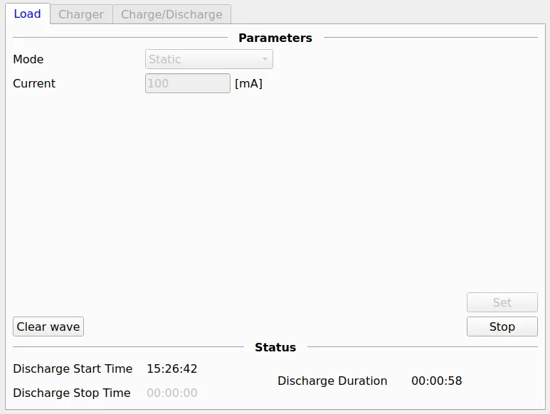
- Select Static in the mode combo.
- Enter the current in mA and press Set. The value is stored in the device; nothing is drawn yet.
- Make sure the load stage is enabled (Load Enabled indicator in the Controls row).
- Press Start. The sink now draws the set current; Stop releases it and Start picks it up again at the same value.
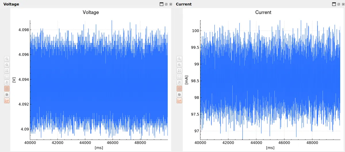
With the acquisition running, the result is immediately visible on the plots. The screenshot below shows a 100 mA static load on a lithium cell: the current sits at 100 mA with the noise of the measurement chain around it, and the cell voltage slowly drops as it discharges.
Standard Waves
Standard Wave mode plays a periodic current shape without any table editing: pick the shape, give it an amplitude and a period, and the GUI computes the steps for you.
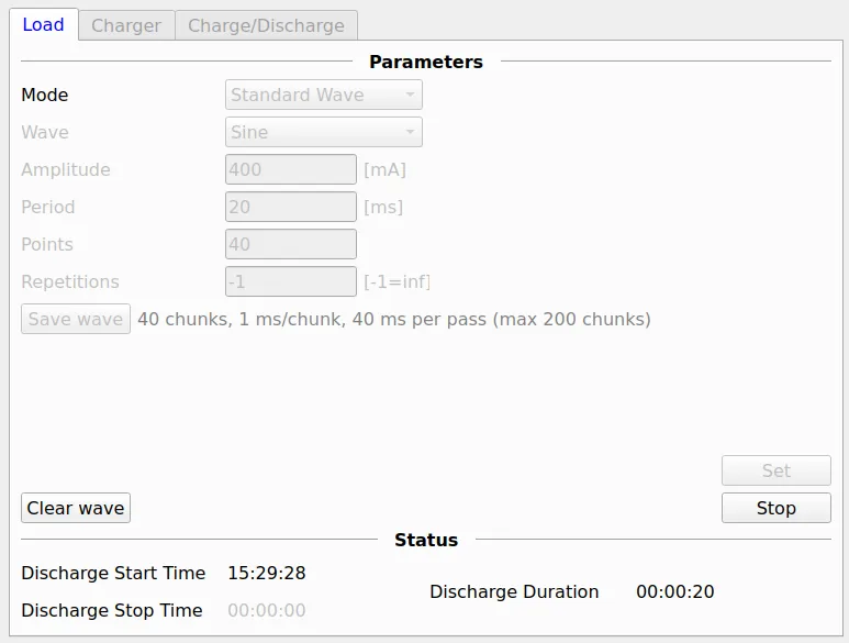
| Field | Meaning |
|---|---|
| Wave | shape: Ramp, Sawtooth, Triangle, Square, Sine |
| Amplitude [mA] | peak current of the shape |
| Period [ms] | duration of one period |
| Points | how many constant-current steps one period is divided into |
| Repetitions | how many periods to play, -1 for endless |
The line next to Save wave tells you what will be sent before you send it: the number of chunks (one per point), the duration of each chunk and of one full pass, against the device limit of 200 chunks per wave. In the screenshot 40 points over 20 ms give 40 chunks of 1 ms.
Press Start to send the wave and start it; the parameters are greyed out while it runs, Stop aborts, and when the last repetition ends the device reports back and the fields unlock. A standard wave is not saved anywhere unless you press Save wave and give it a name — it then appears in the library like any custom wave and can be reused from Custom Wave mode or as a discharge profile.
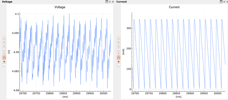
The current plot shows what the probe actually draws:
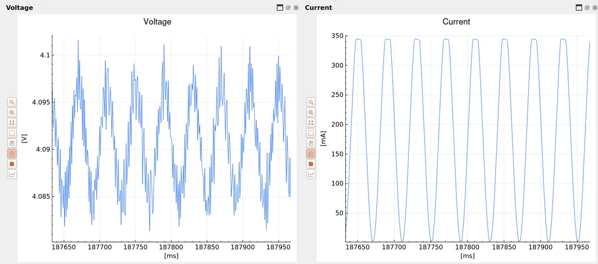
Two things are worth noticing here. The current is built from 40 steps of 1 ms each, and at this zoom the steps are barely visible — with fewer points or longer periods they become a visible staircase, which is expected. And the peak reads about 345 mA for a 400 mA amplitude, which is where the note below comes in.
Custom Waves
Custom Wave mode is where you describe your own current profile. Instead of a shape, you give the device a table of chunks — constant-current steps with a duration — and it plays them one after another. This is the mode to reach for when you want the probe to behave like a real device: a boot phase, a few bursts of activity, an idle tail.
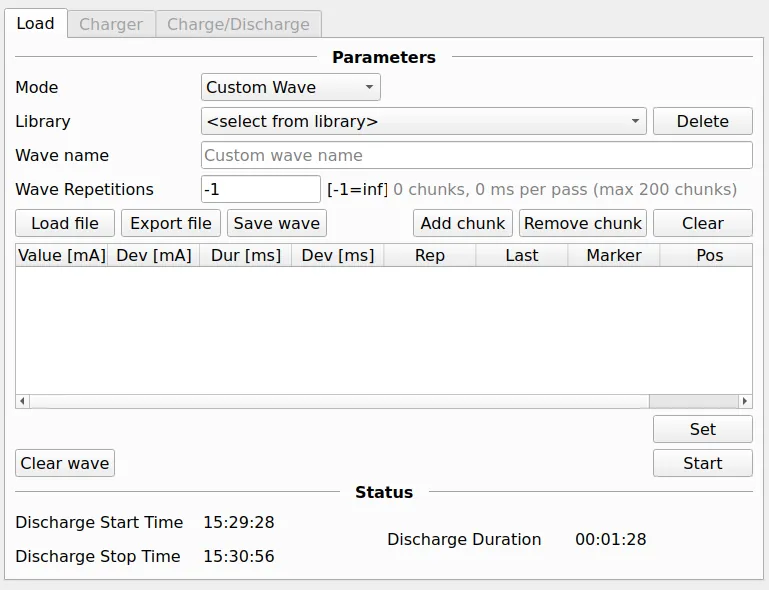
The controls above the table manage the wave as a whole:
- Library – waves you saved earlier; pick one to load it into the table, Delete removes it from the library.
- Wave name – the name used by Save wave.
- Wave Repetitions – how many times the whole table is played,
-1for endless. The line next to it shows the chunk count and the duration of one pass against the 200-chunk device limit. - Load file / Export file – read or write the wave as a text file (see the next section).
- Save wave – store the table in the library under Wave name.
- Add chunk / Remove chunk / Clear – edit the rows.
One row is one chunk:
| Column | Meaning |
|---|---|
| Value [mA] | current of the step |
| Dev [mA] | random ± deviation of the value, drawn again on every play (0 = none) |
| Dur [ms] | duration of the step |
| Dev [ms] | random ± deviation of the duration (0 = none) |
| Rep | how many times this step is repeated back-to-back |
| Last | marks the last chunk of a group; consecutive rows up to it are repeated together |
| Marker | optional energy point name |
| Pos | where the marker goes: s (start), e (end) or s,e (both, two names separated by a comma) |
Groups. Rows up to and including the one with Last checked form a group, and the group is what repeats. For a plain sequential profile you don't need groups at all — just leave Last unchecked and set Wave Repetitions.
Deviations. A non-zero deviation makes the device pick a random value in [value − dev, value + dev] every time the step is played, so a repeated cycle doesn't look identical each time. The randomness is seeded: the same wave gives the same jitter on every run, which keeps measurements comparable.
Markers turn the start and/or end of a step into an energy point on the plots; they are covered in Markers and the Data Analyzer below.
A profile without markers
The wave below reproduces the current of a small WiFi module during one connection cycle: 61 chunks between 70 mA and 410 mA, each a few milliseconds long, played once (Wave Repetitions = 1). It was captured from a real device and typed in as a table — no deviations, no markers.
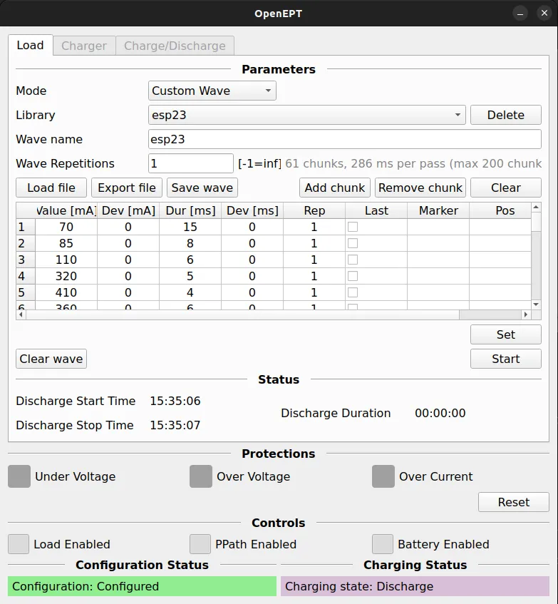
Start the acquisition, press Start, and the profile appears on the current plot exactly as entered:
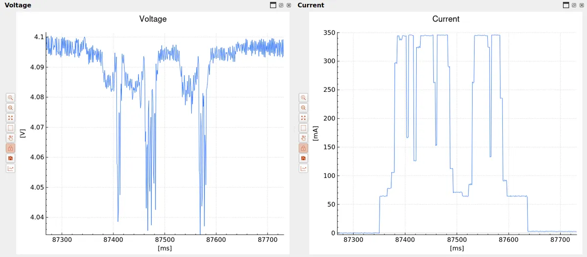
Two details are worth pointing out. The staircase on the way in (65 → 75 → 100 mA) and on the way out (120 → 65 → 80 → 65 mA) matches the table row by row, with steps as short as 4 ms resolved cleanly. And the bursts entered as 410 mA come out flat at about 345 mA — the same ceiling seen with the sine in the previous section — so the highest rows are clipped by the sink rather than reproduced. Keep the profile below that limit if you want the numbers in the table to be the numbers on the plot.
Waveform Library and Wave Files
- Save wave stores the current table (or, in Standard Wave mode, the generated wave) under the name in the Wave name field. Saved waves are kept by the GUI between sessions and listed in the Library combo; select one to load it into the table, Delete removes it. Waves saved from either mode are also offered as discharge profiles on the Charger tab (next section).
- Export file writes the table to a plain text
.txtfile, Load file reads one back. The file is human-readable — it is the list of commands the GUI sends to the device, with a two-line header:
# name: IoT nested 200s
# type: Custom

device wave chunk add -value=5,0,154,0,1,0; -marker="Boot Start" -pos=s
device wave chunk add -value=67,0,350,0,1,0;
device wave chunk add -value=325,0,232,0,1,0; -marker="flash_init" -pos=s
device wave chunk add -value=138,0,1895,0,1,0; -marker="Boot Stop" -pos=e
...
device wave chunk add -value=3,0,2,0,1,1; -marker="FW Stop" -pos=s
device wave counter set -value=1;
This makes long profiles easy to generate with a script and easy to share: the example profiles in Documentation/Waves (a 200 s nested IoT cycle, an LTE tracker, a communication module) were produced that way and can be loaded directly with Load file — the 120-row profile used in the last section of this guide is one of them.
The library itself is a single waveforms.json file in the application data folder of the GUI, so it survives updates and can be copied between machines. Whatever the source, a wave is limited by the device to 200 chunks; the info line next to Wave Repetitions shows the count so you know before pressing Start.
Using a Wave as a Discharge Profile
On the Charge/Discharge tab, the Discharge Profile selector offers Static or any wave from the library. With a library wave selected, a discharge test plays that wave in a loop instead of drawing a flat current, so the battery is discharged with a realistic activity pattern — the device profile from Custom Waves or the IoT cycle from the next section are typical choices. Everything else about the discharge test (thresholds, logging, plots) is unchanged.
For a full discharge, save the wave with Wave Repetitions set to -1 so it loops until the discharge test ends, and rely on the test's cut-off voltage rather than the wave to stop it.
Markers and the Data Analyzer
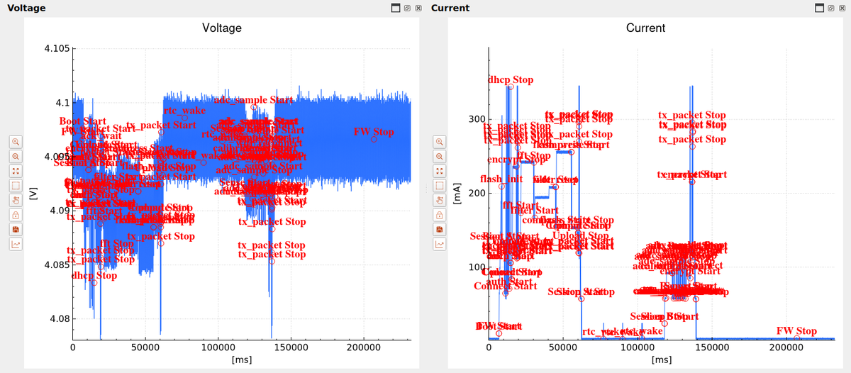
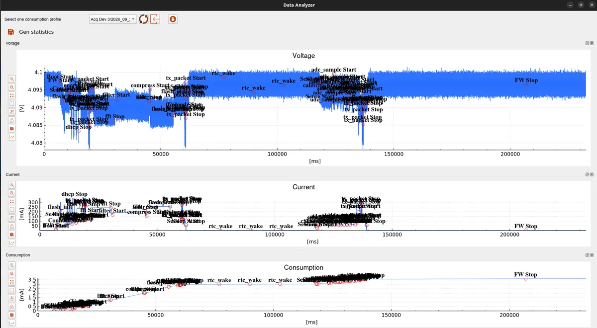
Markers are what turn a replayed current profile into something you can analyse, not just look at. Any chunk can carry a marker at its start, its end, or both, and when the wave plays the probe records an energy point at the exact sample where that chunk boundary happened — the same kind of energy point a real device sends through the FEPLib library. The example below is a 200-second synthetic IoT cycle with three levels of nesting: a firmware run (FW) containing sessions, sessions containing connect / upload / compute / sleep phases, and phases containing individual steps such as tx_packet or fft.
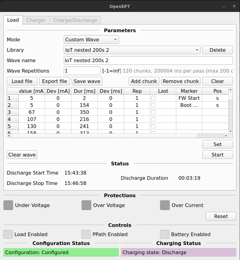
FW and Boot segments with a start marker.Setting markers is a matter of filling the last two columns of the table. Use <name> Start / <name> Stop pairs for anything you want measured as a segment (Boot Start … Boot Stop), nest them freely (Boot inside FW, tx_packet inside Upload), and use a single name without a pair for one-off events such as rtc_wake or flash_init. A chunk can carry both a start and an end marker with s,e and two comma-separated names. The complete profile is available as a wave file in the firmware repository, so you can load it with Load file instead of typing 120 rows.
Start the acquisition first, then press Start on the Load tab. Energy point processing has to be enabled for the acquisition — the GUI warns you if it is not, because the markers would otherwise be lost.
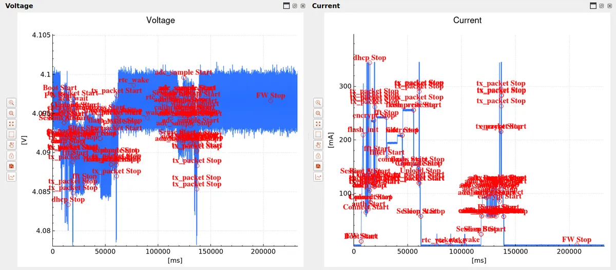
On the live plots each marker appears as a red circle with its name, on the voltage and current plot alike, and the log window lists them as they arrive. With 200-odd markers on a 200 s window the labels overlap, which is expected at this zoom; zooming into any region separates them. What matters here is the placement: because the marker is captured by the probe at the chunk boundary, it sits exactly on the current step, not a few samples off.
Once the acquisition is stopped, the recorded profile can be opened in the Data Analyzer. It shows the same three plots — voltage, current and accumulated consumption — with the markers in place, and the consumption plot now makes the structure obvious: the charge accumulates steeply during the sessions and is flat during sleep.
Gen statistics turns the markers into numbers. Every Start/Stop pair becomes a segment with its start and end time, consumption in mAh, energy in mJ, duration, share of the whole cycle, share of its parent segment and min/max/average current; nested segments are shown as a tree; single markers are listed inside the segment in which they occurred. The coloured bar under the table is the same tree drawn as shares of the cycle, level by level, and the summary lines below it split the recording into marked and unmarked parts. Enter a battery capacity and the tool estimates operating time from the measured cycle; enter a target operating time and it tells you the required capacity.
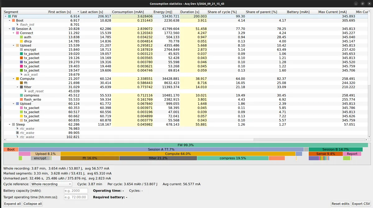
tx_packet costs about 3–5 µAh.For this profile the table answers the questions a firmware engineer would ask before writing the firmware: one 200 s cycle costs 3.65 mAh at an average of 56.6 mA; Compute (fft, filter, compress, flash write) is 64 % of that, Session A as a whole 78 %; the 56 s Sleep phase is 1.3 %; and each tx_packet burst, 40–60 ms at 345 mA, costs 3–5 µAh. Change the wave — shorten the filter, halve the compute — replay it, and the same table shows what the change bought.
Status of the Data Analyzer. The statistics window shown above is work in progress and is not part of this milestone. It is included here only to give an impression of what marker-annotated profiles make possible; column names, layout and features will change before it is released. The Load tab, waveform library, wave files and markers on the live plots described in this guide are complete and available in the current release.