Programmable Load: Firmware, Protocol and GUI Implementation
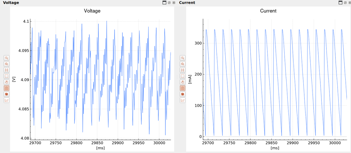
The Energy Profiler Probe (EPP) contains a programmable current sink. Until this milestone it could only be set to a constant value; during Milestone 4 of the second OpenEPT development phase we turned it into a waveform generator that replays an arbitrary current profile, built from chunks with random deviations and embedded energy point markers. This post is the implementation report: how the Load service is organised, how chunks become DAC points and how the timer and DMA drive them, which commands the control protocol gained, and how the GUI Load tab is put together. A companion post, Generating Loads with the Energy Profiler Probe, covers the same feature from the user's side.
In This Update
- Load Service in Firmware – the load mechanism, the service, chunk storage and serialisation, the timer / DMA / DAC path, markers and completion.
- Protocol Description – the
device load,device dacanddevice wavecommands, how they map onto the service, and the status link notification. - GUI – the Load tab, the waveform model and library, and the device command layer.
Load Service in Firmware
The programmable load functionality is implemented through a dedicated Load service in the Energy Profiler Probe firmware. Its role is to provide a single firmware interface for controlling the programmable current sink, including both static current generation and execution of user-defined current waveforms. The service separates the higher-level description of the required load from the low-level hardware operations needed to reproduce it, allowing the same interface to be used by the Control service and, consequently, by the desktop GUI.
The public interface provides functions for configuring the load current and state, controlling the DAC, defining waveform chunks, configuring waveform repetition and randomization, and starting or stopping waveform execution.
Programmable Load Control
At the hardware level, the programmable load is based on an analog current-sink stage whose reference voltage is generated by channel D of the DAC6578. The requested load current is converted by the firmware into the corresponding reference voltage and subsequently into the digital value written to the DAC. In addition to the current set-point, the current-sink stage has a dedicated enable signal controlled through a GPIO.
From the firmware perspective, these functions are intentionally handled independently. The Load service maintains the requested current value, the load enable state, and the DAC state as separate parameters. This makes it possible, for example, to configure a current value before activating the DAC or enabling the load. When the DAC is activated, the previously configured value can immediately be applied to the current-sink stage. The same mechanism is also used when a waveform is executed, with the difference that the DAC value is updated automatically according to the waveform definition.
Service Architecture
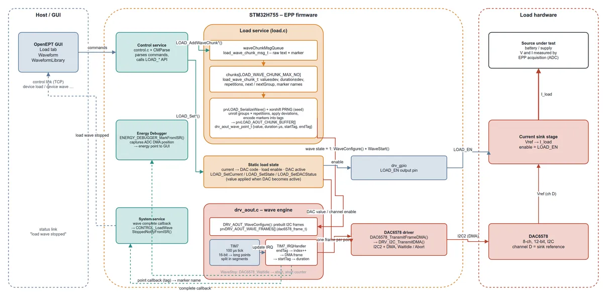
The Load functionality follows the service-oriented organization used throughout the OpenEPT firmware. It is implemented as a dedicated FreeRTOS task and contains its own synchronization objects, message queue, and internal state. Public API functions update the service state and notify the Load task when an operation requiring hardware interaction has to be performed. This keeps the hardware-control sequence inside the Load service and provides a well-defined interface to the remaining firmware components.
The Load service implementation is available in the OpenEPT Firmware repository:
- Load service implementation:
Middlewares/Services/Load/load.c - Load service public interface:
Middlewares/Services/Load/load.h
The service keeps two main data structures. prvLOAD_DATA contains the service-related and static load state, including the configured current, DAC value, load state, requested DAC state, message queue, synchronization objects, and task handle. The waveform itself is maintained separately in prvLOAD_WAVE_DATA, which contains the configured chunks and all information required for waveform generation.
The waveform description is based on the following structures:
typedef struct load_wave_chunk_t
{
    uint32_t id;

    uint32_t baseValue;     /* Base current value in mA */
    uint32_t bsDev;         /* ± current deviation */

    uint32_t duration;      /* Duration in ms */
    uint32_t dDev;          /* ± duration deviation */

    int      maxRepetitionCnt;
    uint32_t lastInGroup;

    char     markerStartName[LOAD_WAVE_MARKER_NAME_SIZE];
    char     markerEndName[LOAD_WAVE_MARKER_NAME_SIZE];

    struct load_wave_chunk_t* next;       /* Next chunk in the same group */
    struct load_wave_chunk_t* nextGroup;  /* First chunk of the next group */

} load_wave_chunk_t;

typedef struct
{
    load_wave_chunk_t  chunks[LOAD_WAVE_CHUNK_MAX_NO];

    uint32_t           waveChunksCounter;

    load_wave_chunk_t* firstInChain;
    load_wave_chunk_t* last;

    load_wave_state_t  state;
    int                repetitionCounter;

    uint32_t           seed;
    uint32_t           rngState;

} load_wave_data_t;
Chunks are stored in a statically allocated array and linked into groups. The next pointer connects chunks belonging to the same group, while nextGroup connects the last chunk of one group, identified by lastInGroup = 1, with the first chunk of the following group. This representation allows the waveform to preserve its logical organization while avoiding dynamic memory allocation. The static allocation provides a hard upper bound defined by LOAD_WAVE_CHUNK_MAX_NO and deterministic memory usage, which is important because the Load service operates concurrently with the acquisition and communication parts of the firmware.
From Chunk Command to DAC Point
Waveforms are not transferred to the firmware as a complete array of DAC samples. They are built up incrementally from compact waveform chunks, and each chunk passes through a fixed pipeline of stages before it reaches the DAC. The diagram below shows that pipeline from left to right: what enters each stage, what the stage does, what leaves it, and which task or context owns it.
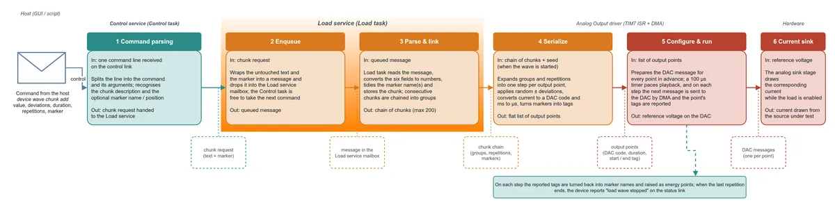
1 – Command parsing (Control task). A device wave chunk add line arrives on the control link. CMParse splits the command from its arguments and the handler prvCONTROL_AddWaveChunk() reads -value, the optional -marker and -pos. It does not interpret the six numeric fields; it only forwards the raw text.
2 – Enqueue (Control → Load task). LOAD_AddWaveChunkWithMarker() copies the description and the marker into a load_wave_chunk_msg_t and posts it on waveChunkMsgQueue. The Control task returns immediately and can serve the next command while the Load task does the work.
value,valueDeviation,duration,durationDeviation,repetition,lastInGroup3 – Parse and link (Load task). The Load task drains the queue, parses the six fields, trims the marker name(s) — with -pos=s,e there are two, separated by a comma — and fills a load_wave_chunk_t in the static chunks[] array. The chunk is linked to its predecessor through next, or through nextGroup when the previous chunk closed a group with lastInGroup = 1. The chunk stays in this compact form until the wave is started, so a 200-chunk wave costs 200 structures, not 200 × repetitions.
4 – Serialize (Load task, on device wave state set -value=1). The chunk chain is unrolled into a flat point buffer, which is the representation the driver needs for real-time playback:
typedef struct
{
    uint16_t value;      /* DAC code */
    uint32_t duration;   /* Duration in µs */
    uint32_t startTag;   /* Event reported when the point starts */
    uint32_t endTag;     /* Event reported when the point ends */
} drv_aout_wave_point_t;

static drv_aout_wave_point_t prvLOAD_AOUT_CHUNK_BUFFER[LOAD_AOUT_MAX_CHUNKS];
Walking from firstInChain, every chunk is emitted maxRepetitionCnt times. For each emitted point the current is jittered by its deviation (next section), converted to the sink reference voltage and then to a DAC code, and the duration is jittered and converted from milliseconds to microseconds:
static float prvLOAD_CurrentToVoltage(uint32_t current)
{
    return ((float)current / 1000.0f) * 8.8f * 0.075f;
}
Markers become tags: the chunk id is written into startTag of the first emitted point and, with the end flag set, into endTag of the last one.
5 – Configure and run (Analog Output driver). DRV_AOUT_WaveConfigure() receives the point buffer and prebuilds one complete DAC6578 I2C frame per point, so nothing has to be computed later in interrupt context. DRV_AOUT_WaveStart() writes the first point and starts TIM7; from then on the timer interrupt ends the current point, reports its endTag, pushes the next frame to the DAC through I2C DMA and reports the next startTag. Tags come back to the Load service, which resolves them to marker names and raises energy points; the last repetition raises the complete callback that ends in the load wave stopped status message.
6 – Current sink (hardware). DAC channel D provides the reference for the analog sink stage, which draws the corresponding current from the source under test as long as LOAD_EN is active.
The division of labour is deliberate: the Control task only moves text, the Load task owns every waveform structure and does all conversions in task context, and the driver's interrupt handler only ever touches precomputed data.
Randomized Current and Duration
The waveform format allows both the current value and duration of a chunk to contain a configurable random deviation. These deviations are applied during serialization rather than while the waveform is being executed.
For every generated point, the Load service calculates:
current  = baseValue ± bsDev
duration = duration  ± dDev
A deterministic pseudo-random generator is used to generate these deviations. Its state is initialized from the configurable waveform seed at the beginning of every serialization. Consequently, the same waveform definition combined with the same seed produces exactly the same sequence of randomized current values and durations.
This behavior is particularly useful for repeatable experiments. A load profile can contain controlled variations that better approximate real application behavior while still allowing the identical waveform to be reproduced when comparing different firmware implementations, hardware configurations, or energy-management algorithms.
Energy Marker Integration
Each waveform chunk can optionally define an Energy Debugger marker at its beginning, its end, or both. During serialization, these markers are encoded into the startTag and endTag fields of the corresponding drv_aout_wave_point_t.
A start marker is associated with the first generated point of the corresponding chunk, while an end marker is associated with its last generated point. The Analog Output driver treats these tags as opaque values and reports them through a callback when the corresponding waveform boundary is reached.
The Load service then resolves the tag back to the original chunk and generates the corresponding Energy Debugger event:
ENERGY_DEBUGGER_MarkFromISR(
    chunk->markerStartName,
    chunk->markerStartNameSize
);
or:
ENERGY_DEBUGGER_MarkFromISR(
    chunk->markerEndName,
    chunk->markerEndNameSize
);
This integrates generated load waveforms directly with the existing OpenEPT energy-debugging infrastructure. From the acquisition and analysis perspective, an energy point generated by the Load service is handled in the same way as an energy point originating from a device under test.
Waveform Execution
Once the wave has been serialized, the flat list of output points is handed to the Analog Output driver, which owns the time-critical part: stepping the DAC through the points at the right moments. Two design choices keep that part small and deterministic. First, all DAC communication frames are prepared before playback starts, one per point, so nothing has to be assembled while the wave is running. Second, timing and data transfer are split between two peripherals: TIM7 decides when a point ends, and I2C DMA moves the next frame to the DAC without any blocking transaction in the interrupt handler.
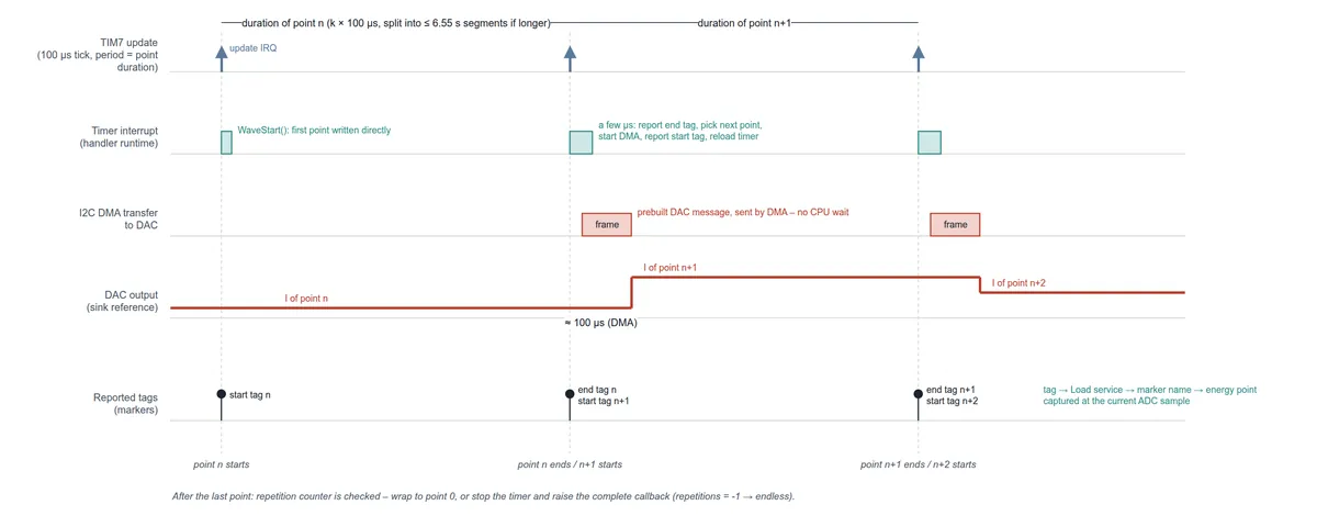
Playback starts with the first point written to the DAC directly and TIM7 loaded with that point's duration. From then on every point boundary is handled the same way inside the timer interrupt: the end tag of the finished point is reported, the driver moves to the next point, its prebuilt frame is queued for DMA, its start tag is reported, and the timer is reloaded with the new duration. The handler itself runs for a few microseconds; the DAC output actually changes when the DMA transfer completes, a fixed and short delay after the tick, so the step-to-step timing depends only on the timer.
The sequence repeats until the last point has been played. The driver then checks the repetition counter: if further repetitions remain it wraps back to the first point without stopping the timer, otherwise it stops TIM7 and raises the completion callback. A repetition count of -1 means the wave is played continuously until it is stopped.
Long-Duration Points
The waveform timing mechanism also supports load states whose duration exceeds the maximum period that can be represented directly by TIM7. Instead of requiring the waveform definition to split such intervals into multiple artificial chunks, the Analog Output driver internally divides a long duration into several timer segments.
From the Load service perspective, the interval remains a single waveform point. The timer interrupt consumes the required segments until the complete duration has elapsed and only then advances to the next waveform point.
This is particularly useful when generating realistic battery-powered embedded-system profiles, where short active phases may be followed by sleep intervals lasting several seconds or minutes.
Waveform Completion
When all waveform points and configured repetitions have been executed, the Analog Output driver invokes the completion callback registered by the Load service. The Load service then changes its internal waveform state back to LOAD_WAVE_STATE_INACTIVE and forwards the completion event through the registered service callback.
The System service connects this callback to the Control service, which sends a:
load wave stoppedstatus notification to the GUI.
Protocol Description
All load functionality is exposed through the existing text protocol on the control link. Commands are registered in the Control service with CMPARSE_AddCommand() and parsed by CMParse.
- Command handlers:
Middlewares/Services/Control/control.c(prvCONTROL_SetLoadCurrent,prvCONTROL_AddWaveChunk,prvCONTROL_WaveChunkSet, …) - Argument parser (quoted values, NUL termination):
Middlewares/Services/Control/CMParse/cmparse.c - Status link message:
CONTROL_LoadWaveStoppedNotifyFromISR()incontrol.c - Example wave files:
Documentation/Waves
Static load and DAC
| Command | Service call | Effect |
|---|---|---|
device load current set -value=<mA> |
LOAD_SetCurrent() |
store set-point; applied immediately only if DAC active |
device load current get |
LOAD_GetCurrent() |
returns stored set-point |
device load enable / device load disable |
LOAD_SetState() |
enable GPIO of the sink stage |
device load get |
LOAD_GetState() |
enable state |
| `device dac enable set -value=<0\ | 1>` | LOAD_SetDACStatus() |
device dac enable get |
LOAD_GetDACStatus() |
|
device dac value set -value=<code> / get |
LOAD_SetDACValue() / LOAD_GetDACValue() |
raw 12-bit code, used by calibration |
Wave
| Command | Service call | Effect |
|---|---|---|
| `device wave chunk add -value=v,vDev,dur,durDev,rep,last [-marker="…" -pos=s\ | e\ | s,e]` |
| `device wave counter set -value=<n\ | -1>` | LOAD_SetWaveCounter() |
device wave seed set -value=<seed> |
LOAD_SetWaveSeed() |
PRNG seed for deviations |
| `device wave state set -value=<0\ | 1>` | LOAD_SetWaveState() |
device wave clear |
LOAD_ClearWave() |
drop all chunks (required before loading another wave) |
A chunk line always follows the same six-field order; the marker part is optional. With -pos=s,e the marker value carries two comma-separated names, start first:
device wave chunk add -value=468,0,22,0,1,0; -marker="tx_packet Start, tx_packet Stop" -pos=s,eThe intended sequence from a client is therefore: device wave clear → n × device wave chunk add → device wave counter set → (device wave seed set) → device wave state set -value=1, and device wave state set -value=0 to abort. The DAC is activated by the service when the wave starts; device load enable still controls the physical stage.
Status link notification
When the last repetition ends the device sends, unsolicited, on the status link:
load wave stoppedas an action message (type byte 1). The GUI listens for it to restore the Start/Stop buttons and the wave state; nothing is sent for a stop requested by the client, since the client already knows.
A note on the parser
Supporting -marker="a name with spaces" required quoted values in CMParse. While adding them we found that parsed values were not NUL-terminated and that some Control handlers reuse one cmparse_value_t for several arguments; with the right lengths a stale character from the previous value could survive, which showed up as a wrong sampling prescaler on the device. The parser now always terminates values and bounds the copy; the lesson was cheap to fix and expensive to find, so it is recorded here.
GUI
On the GUI side the whole feature lives in the Load tab of the device window. The tab has one Mode selector with three entries — Static, Standard Wave and Custom Wave — and the parameter area below it changes with the mode. The row at the bottom is shared by all modes: Set and Start/Stop on the right, Clear wave on the left.
- Load tab (modes, chunk table, library, file import/export, Clear/Start/Stop):
Windows/Device/energycontrolwnd.cpp,energycontrolwnd.h - Waveform model and library (
Waveform,WaveformLibrary, wave file format):Processing/waveform.cpp,waveform.h - Device command layer (
setLoadCurrent,setLoadWave,setLoadWaveState,clearLoadWave,sigLoadWaveStopped):device.cpp,device.h - Window ↔ device glue:
devicecontainer.cpp - Charger/Discharge tab (library wave as discharge profile):
Windows/Device/energycontrolwnd.cpp(chdischDischargeStart/Stop)
Static mode
Static mode is the direct front end for the three load operations described in the firmware section: a current entry with Set (stores the set-point in the device), the Load enable, and Start/Stop, which activates and deactivates the DAC. Because the value is stored separately from the DAC state, the three can be used in any order and a discharge can be stopped and resumed at the same current.
Standard Wave mode
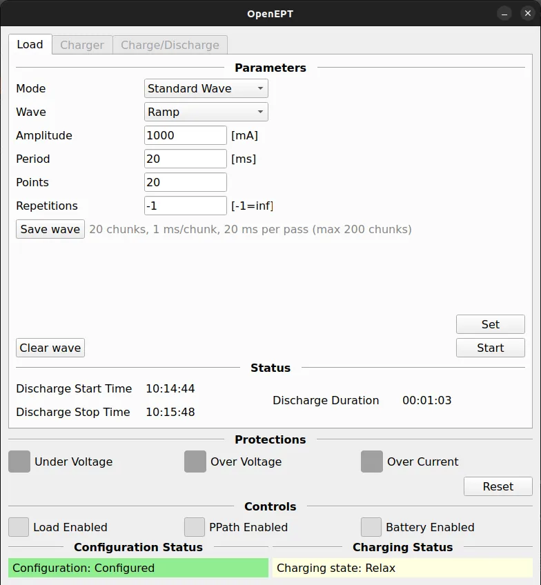
Standard Wave generates a periodic current from a handful of parameters, all computed locally in the GUI before anything is sent:
- Wave – the shape: Ramp, Sawtooth, Triangle, Square or Sine.
- Amplitude [mA] – peak current of the shape.
- Period [ms] – duration of one period.
- Points – how many constant-current steps one period is divided into; each step becomes one chunk, so the info line next to Save wave reports the resulting chunk count, duration per chunk and duration per pass against the device limit of 200 chunks.
- Repetitions – how many periods are played;
-1plays until Stop.
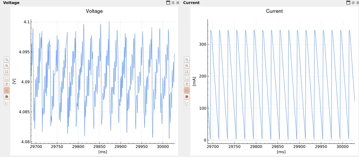
Start sends the generated chunk list, the repetition counter and the start command; the wave is not stored anywhere unless Save wave is pressed, which puts it into the waveform library under a name so it can be reused from Custom Wave mode or as a discharge profile.
Custom Wave mode
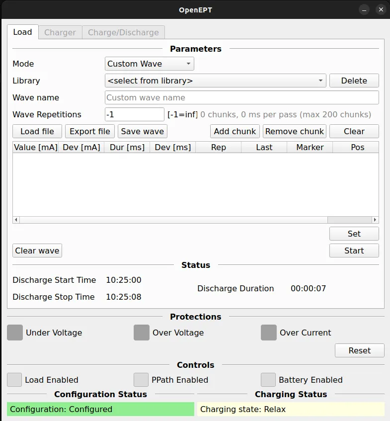
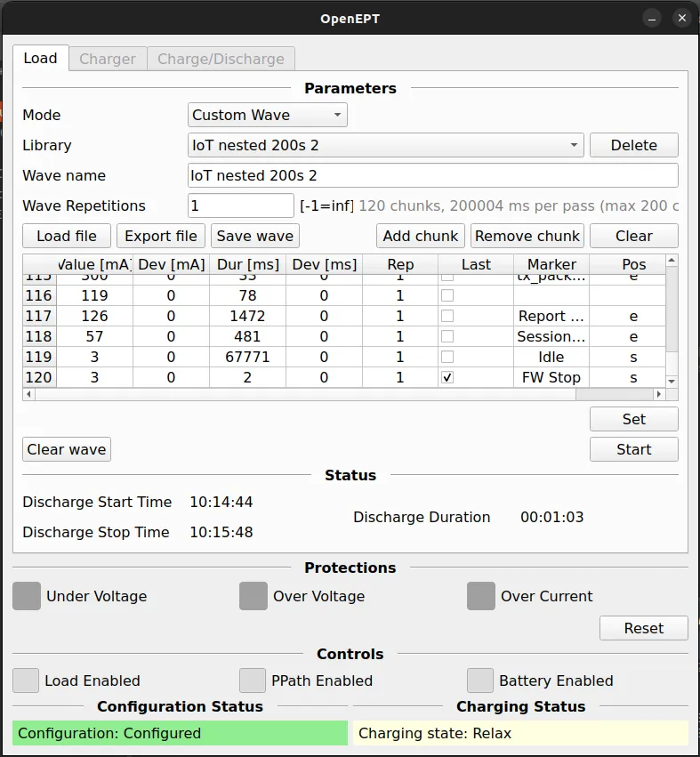
Custom Wave exposes the chunk model of the firmware one to one. The controls above the table manage the wave as a whole:
- Library – waves saved earlier; selecting one fills the table, Delete removes it from the library.
- Wave name – the name under which Save wave stores the current table in the library.
- Wave Repetitions – how many times the whole wave is played (
-1= endless); the info line next to it shows the chunk count, the duration of one pass and the device limit. - Load file / Export file – read or write the wave as a plain text file.
- Save wave – store the table in the library.
- Add chunk / Remove chunk / Clear – edit the rows of the table.
Each row of the table is one chunk, i.e. one constant-current step, and the columns map directly onto the fields of the chunk command sent to the device:
| Column | Meaning |
|---|---|
| Value [mA] | current of the step |
| Dev [mA] | random ± deviation applied to the value on every play (0 = none) |
| Dur [ms] | duration of the step |
| Dev [ms] | random ± deviation applied to the duration (0 = none) |
| Rep | how many times the step is repeated back-to-back |
| Last | marks the last chunk of a group; consecutive rows up to it are repeated together |
| Marker | optional energy point name |
| Pos | where the marker is placed: s (start of the chunk), e (end) or s,e (both; two names separated by a comma) |
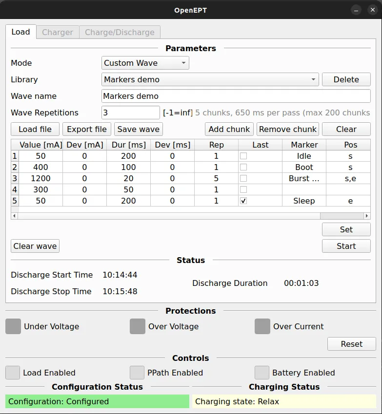
Marker positions are normalised and validated before the wave is sent. Starting a wave that carries markers while energy point processing is disabled for the acquisition raises a warning, since the markers would be lost silently.
Waveform model
Waveform is the single in-memory representation used by every part of the GUI:
typedef struct
{
    unsigned int value;         unsigned int valueDev;
    unsigned int duration;      unsigned int durationDev;
    int          repetitions;   bool         lastInGroup;
    QString      marker;        QString      markerPos;   // "s", "e", "s,e"
} waveform_chunk_t;

class Waveform
{
    bool        generateStandard(waveform_type_t type, unsigned int amplitude, unsigned int period, unsigned int points, int repetitionCounter);
    QStringList getCommands();                         // chunk lines + counter set
    bool        parseContent(QString content, QString* error);
    bool        loadFromFile(QString path, QString* error);
    bool        saveToFile(QString path, QString* error);
    QJsonObject toJson();  bool fromJson(QJsonObject obj);
    static QString chunkToCommand(waveform_chunk_t chunk);
    static bool    chunkFromCommand(QString line, waveform_chunk_t* chunk);
    ...
};
The important design decision is that chunkToCommand() / chunkFromCommand() are the only serialisation: the wave file format on disk is literally the command list with a two-line header, and what is sent to the device is the same list. There is no second format to keep in sync, and a file generated by a script (the profiles in Documentation/Waves were produced that way) is directly loadable.
WaveformLibrary is a singleton that persists waves as JSON in the application data folder (waveforms.json), distinguishes standard from user waves (waveform_origin_t), and emits sigLibraryChanged() so that every combo box showing library waves (Load tab, Discharge Profile selector) refreshes.
Device command layer
Device exposes the wave as three operations: setLoadWave(Waveform) sends device wave clear, every chunk line and the counter; setLoadWaveState(bool) sends device wave state set; clearLoadWave() sends device wave clear. setLoadCurrent() maps to device load current set. Responses are handled like every other control command (a STATUS/ERROR line). On the status link, onStatusLinkNewMessageReceived() recognises the load wave stopped action message and emits sigLoadWaveStopped(), which DeviceContainer forwards to the window (loadWaveStopped()) to re-enable Start.
The Charger/Discharge tab reuses all of this: its Discharge Profile selector offers Static or any library wave, and a discharge with a library wave is just setLoadWave() + setLoadWaveState(true) with the load enabled.
What Comes Next
Two things are already on the list. Deviations are currently applied once, at serialisation, so every repetition of the wave gets the same jitter; moving deviation generation into the driver (one chunk = one point, jitter applied when the point is loaded) would give every repetition its own and would remove the unroll buffer altogether. And the standard wave generator will get the same per-chunk deviation fields the custom table already has.